Crashteroseismology

A quick timeout

The examples on this page assume that the user already has some basic-level experience with Python and therefore if not, we highly recommend that you first visit the Python website and going through some of their tutorials before attempting ours.

We will work through two examples – each demonstrating a different application of the software. The first example will run pySYD as a script from command line since this is what it was optimized for. We will break down each step of the software as much as possible with the hope that it will provide a nice introduction to both the software and science. For the second one, we will reconstruct everything in a more condensed version and show pySYD imported and used as a module.

If you have any questions, check out our user guide for more information. If this still does not address your question or problem, please do not hesitate to contact Ashley directly.

---

A crash course in asteroseismology

For purposes of this first example, we’ll assume that we don’t know anything about the star or its properties so that the software runs from start to finish on its own. In any normal circumstance, however, we can provide additional inputs like the center of the frequency range with the oscillations, or numax ( \(\rm \nu_{max}\)), that can bypass steps and save time.

Initialize script

When running pySYD from command line, you will likely use something similar to the following command:

pysyd run --star 1435467 -dv --ux 5000 --mc 200

which we will now deconstruct.

pysyd

if you used pip install, the binary (or executable) should be available. In fact, the setup file defines the entry point for pysyd, which is accessed through the pysyd.cli.main script – where you can also find all available parsers and commands

run

regardless of how you choose to use the software, the most common way you will likely implement pySYD is in run mode – which, just as it sounds, will process stars in order. This is saved to the args parser NameSpace as the mode, which will run the pipeline by calling pysyd.pipeline.run. There are currently five available (tested) modes (with two more in development), all which are described in more detail here

--star 1435467

here we are running a single star, KIC 1435467. You can also provide multiple targets, where the stars will append to a list and then be processed consecutively. On the other hand, if no targets are provided, the program would default to reading in the star or todo list (via info/todo.txt). Again, this is because the software is optimized for running many stars.

-dv

adapting Linux-like behavior, we reserved the single hash options for booleans which can all be grouped together (as shown above). Here the -d and -v are short for display and verbose, respectively, and show the figures and verbose output. For a full list of options available, please see our command-line glossary. There are dozens of options to make your experience as customized as you’d like!

--ux 5000

this is an upper frequency limit for the first module that identifies the power eXcess due to solar-like oscillations. In this case, there are high frequency artefacts that we would like to ignore. We actually made a special notebook tutorial specifically on how to address and fix this problem. If you’d like to learn more about this or are having a similar issue, please visit this page.

--mc 200

last but certainly not least - the mc (for Monte Carlo-like) option sets the number of iterations the pipeline will run for. In this case, the pipeline will run for 200 steps, which allows us to bootstrap uncertainties on our derived properties.

Note: For a complete list of options which are currently available via command-line interface (CLI), see our special CLI glossary.

The steps

The software operates in roughly the following steps:

1. Load in parameters and data

2. Search and estimate initial values

3. Select best-fit stellar background model

4. Fit global parameters

5. Estimate uncertainties

For each step, we will first show the relevant block of printed (or verbose) output, then describe what the software is doing behind the scenes and if applicable, conclude with the section-specific results (i.e. files, figures, etc.).

Warning

Please make sure that all input data are in the correct units in order for the software to provide reliable results. If you are unsure, please visit this page for more information about formatting and input data.

1. Load in parameters and data

-----------------------------------------------------------
Target: 1435467
-----------------------------------------------------------
# LIGHT CURVE: 37919 lines of data read
# Time series cadence: 59 seconds
# POWER SPECTRUM: 99518 lines of data read
# PS oversampled by a factor of 5
# PS resolution: 0.426868 muHz
-----------------------------------------------------------

During this step, it will take the star name along with the command-line arguments and create an instance of the pysyd.target.Target object. Initialization of this class will automatically search for and load in data for the given star, as shown in the output above. Both the light curve and power spectrum were available for KIC 1435467 and as you can see in these cases, pySYD will use both arrays to compute additional information like the time series cadence, power spectrum resolution, etc.

If there are issues during the first step, pySYD will flag this and immediately halt any further execution of the code. If something seems questionable during this step but is not fatal for executing the pipeline, it will only return a warning. In fact, all pysyd.target class instances will have an ok attribute - literally meaning that the star is ‘ok’ to be processed. By default, the pipeline checks this attribute before moving on.

Since none of this happened, we can move on to the next step.

2. Search and estimate initial values

-----------------------------------------------------------
PS binned to 228 datapoints

Numax estimates
---------------
Numax estimate 1: 1440.07 +/- 81.33
S/N: 2.02
Numax estimate 2: 1513.00 +/- 50.26
S/N: 4.47
Numax estimate 3: 1466.28 +/- 94.06
S/N: 9.84
Selecting model 3
-----------------------------------------------------------

The main thing we need to know before performing the global fit is an approximate starting point for the frequency corresponding to maximum power, or numax (\(\rm \nu_{max}\)). Please read the next section for more information regarding this.

The software first makes a very rough approximation of the stellar background by binning the power spectrum in both log and linear spaces (think a very HEAVY smoothing filter), which the power spectrum is then divided by so that we are left with very little residual slope in the PS. The ‘Crude Background Fit’ is shown below in the second panel by the lime green line. The background-corrected power spectrum (BCPS) is shown in the panel to the right.

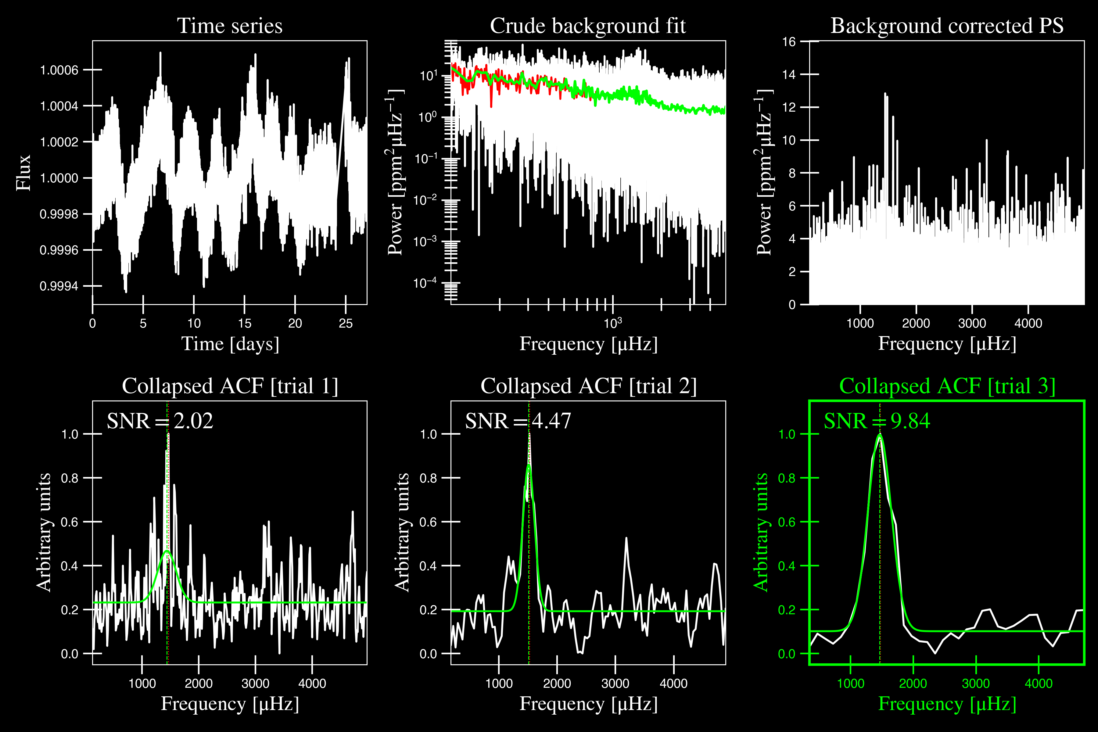
Next pySYD uses a “collapsed” autocorrelation function (ACF) technique with different bin sizes to identify localized power excess in the PS due to solar-like oscillations. By default, this is done three times (or trials) and hence, provides three different estimates - which is typically sufficient for these purposes. The bottom row in the above figure shows these three trials, highlighting the one that was selected, or the one with the highest signal-to-noise (S/N).

Finally, it saves the best estimates in a csv file for later use, which can be used to bypass this step the next time that the star is processed.

1435467 parameter estimates

stars	numax	dnu	snr
1435467	1466.27585610943	73.4338977674559	9.84295865829856

3. Select best-fit stellar background model

-----------------------------------------------------------
GLOBAL FIT
-----------------------------------------------------------
PS binned to 333 data points

Background model
----------------
Comparing 6 different models:
Model 0: 0 Harvey-like component(s) + white noise fixed
 BIC = 981.66 | AIC = 2.95
Model 1: 0 Harvey-like component(s) + white noise term
 BIC = 1009.56 | AIC = 3.02
Model 2: 1 Harvey-like component(s) + white noise fixed
 BIC = 80.27 | AIC = 0.22
Model 3: 1 Harvey-like component(s) + white noise term
 BIC = 90.49 | AIC = 0.24
Model 4: 2 Harvey-like component(s) + white noise fixed
 BIC = 81.46 | AIC = 0.20
Model 5: 2 Harvey-like component(s) + white noise term
 BIC = 94.36 | AIC = 0.23
Based on BIC statistic: model 2
-----------------------------------------------------------

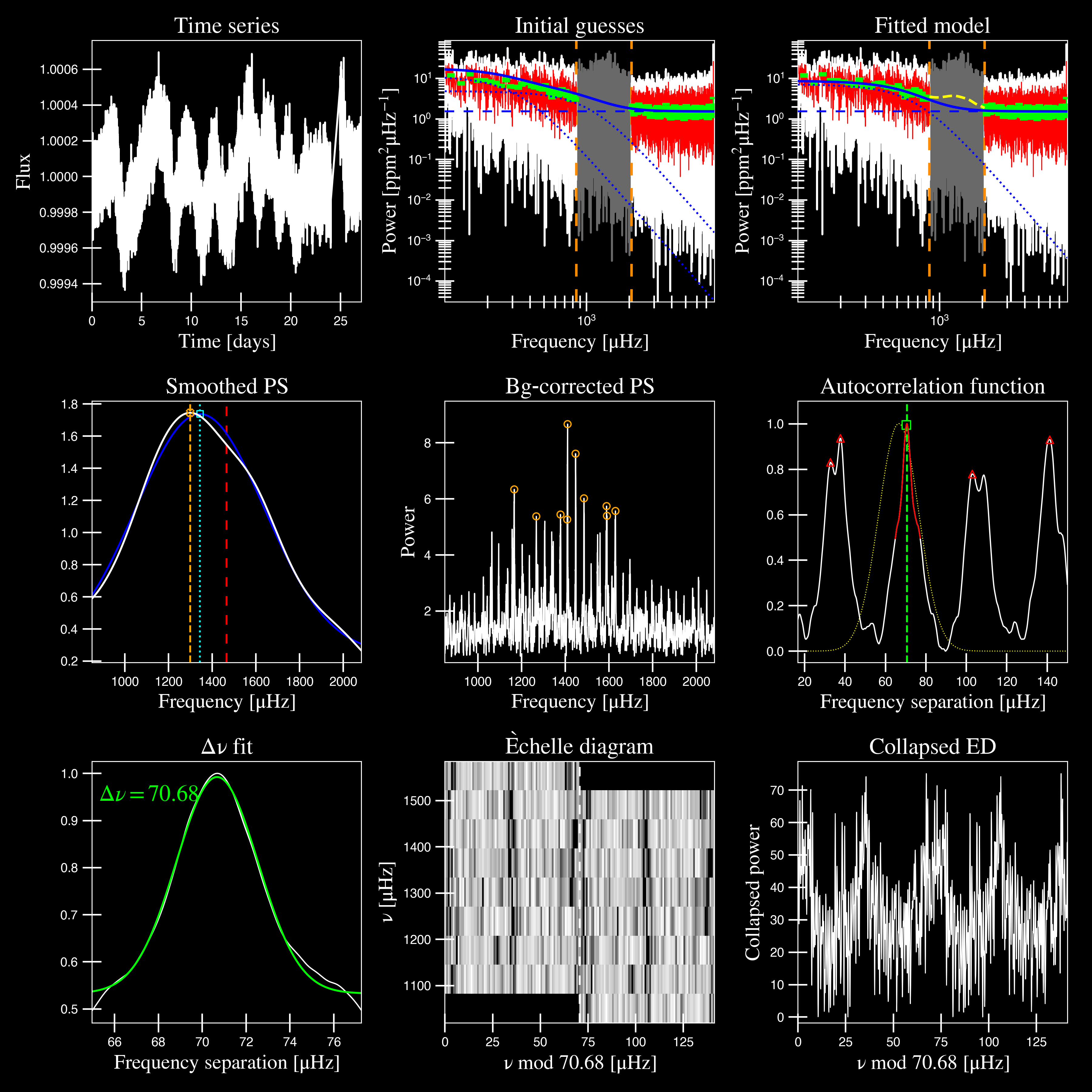
A bulk of the heavy lifting is done in this main fitting routine, which is actually done in two separate steps: 1) modeling and characterizing the stellar background and 2) determining the global asteroseismic parameters. We do this separately in two steps because they have fairly different properties and we wouldn’t want either of the estimates to be influenced by the other in any way.

Ultimately the stellar background has more of a “presence” in the power spectrum in that, dissimilar to solar-like oscillations that are observed over a small range of frequencies, the stellar background contribution is observed over all frequencies. Therefore by attempting to identify where the oscillations are in the power spectrum, we can mask them out to better characterize the background.

We should take a sidestep to explain something important that is happening behind the scenes. A major reason why the predecessor to pySYD, IDL-based SYD, was so successful was because it assumed that the estimated numax and granulation timescales could be scaled with the Sun – a fact that was not known at the time but greatly improved its ability to quickly and efficiently process stars. This is clearly demonstrated in the 2nd and 3rd panels in the figure below, where the initial guesses are strikingly similar to the fitted model.

While this scaling relation ensured great starting points for the background fit, SYD still required a lot fine-tuning by the user. Therefore we adapted the same approach but instead implemented an automated background model seletion. After much trial and error, the BIC seems to perform better for our purposes - which is now the default metric used (but can easily be changed, if desired).

Measuring the granulation time scales is obviously limited by the total observation baseline of the time series but in general, we can resolve up to 3 Harvey-like components (or laws) at best (for now anyway). For more information about the Harvey model, please see the original paper 1 as well as its application in context .

Therefore we use all this information to guess how many we should observe and end up with

\[n_{\mathrm{models}} = 2 \cdot (n_{\mathrm{laws}}+1)\]

models for a given star. The fact of 2 is because we give the options to fix the white noise or for it to also be a free parameter. The +1 (times 2) is because we also want to consider the simplest model i.e. where we are not able to resolve any. From our perspective, the main purpose of implementing this was to try to identify null detections, since we do not expect to observe oscillations in every star. However, this is a work in progress and we are still trying various methods to identify and quantify non-detections. Therefore if you have any ideas, please reach out to us!

For this example we started with two Harvey-like components but the automated model selection preferred a simpler one consisting of a single Harvey law. In addition, the white noise was fixed and not a free parameter and hence, the final model had 3 less parameters than it started with. For posterity, we included the output if only a single iteration had been run (which we recommend by default when analyzing a star for the first time).

Note

For more information about what each panel is showing in any of these figures, please visit this page.

4. Fit global parameters

If this was executed with its default mc setting (== 1, for a single iteration), the output parameters would look like that shown below. In fact, we encourage folks to run new stars for a single step first (*ALWAYS*) before running it several iterations to make sure everything checks out.

-----------------------------------------------------------
Output parameters
-----------------------------------------------------------
numax_smooth: 1299.81 muHz
A_smooth: 1.74 ppm^2/muHz
numax_gauss: 1344.46 muHz
A_gauss: 1.50 ppm^2/muHz
FWHM: 294.83 muHz
dnu: 70.68 muHz
tau_1: 234.10 s
sigma_1: 87.40 ppm
-----------------------------------------------------------
 - displaying figures
 - press RETURN to exit
 - combining results into single csv file
-----------------------------------------------------------

Reminder: the printed output above is for posterity. Please see the next section in the event that you are comparing outputs to test the software functionality.

The parameters are printed and saved in identical ways (sans the uncertainties).

1435467 global parameters

parameter	value	uncertainty
numax_smooth	1299.81293631	–
A_smooth	1.74435577479371	–
numax_gauss	1344.46209203309	–
A_gauss	1.49520571806361	–
FWHM	294.828524961042	–
dnu	70.6845197924864	–
tau_1	234.096929937095	–
sigma_1	87.4003388623678	–

5. Estimate uncertainties

-----------------------------------------------------------
Sampling routine:
100%|███████████████████████████████████████| 200/200 [00:21<00:00,  9.23it/s]
-----------------------------------------------------------
Output parameters
-----------------------------------------------------------
numax_smooth: 1299.81 +/- 56.64 muHz
A_smooth: 1.74 +/- 0.19 ppm^2/muHz
numax_gauss: 1344.46 +/- 41.16 muHz
A_gauss: 1.50 +/- 0.24 ppm^2/muHz
FWHM: 294.83 +/- 64.57 muHz
dnu: 70.68 +/- 0.82 muHz
tau_1: 234.10 +/- 23.65 s
sigma_1: 87.40 +/- 2.81 ppm
-----------------------------------------------------------
 - displaying figures
 - press RETURN to exit
 - combining results into single csv file
-----------------------------------------------------------

Notice the difference in the printed parameters this time - which now have uncertainties!

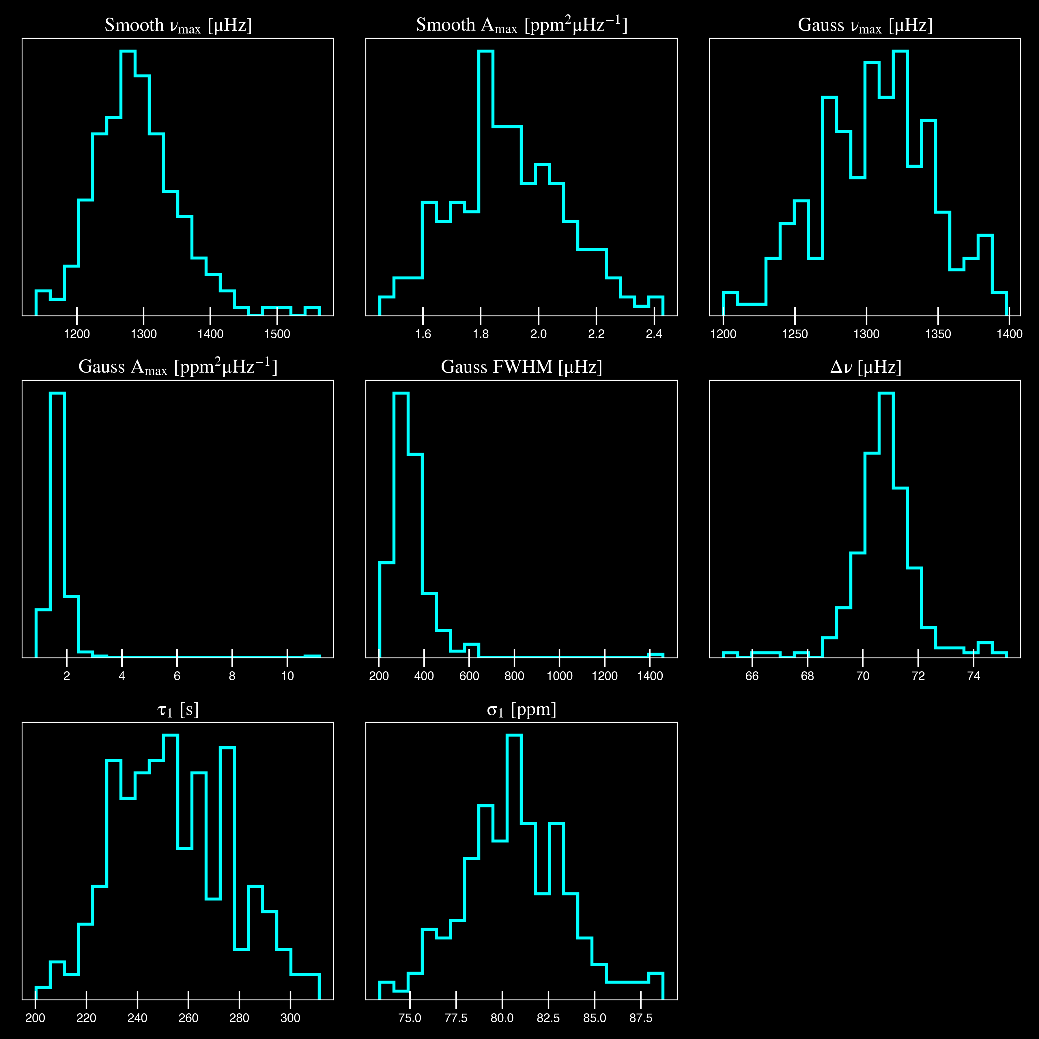
^^ The figure above shows parameter posteriors for KIC 1435467. Sampling results can be saved by using the boolean flag -z or --samples, which will store the samples for the fitted parameters as comma-separated values using pandas.

1435467 global parameters

parameter	value	uncertainty
numax_smooth	1299.81293631	56.642346824238
A_smooth	1.74435577479371	0.191605473120388
numax_gauss	1344.46209203309	41.160592041828
A_gauss	1.49520571806361	0.236092716197938
FWHM	294.828524961042	64.57265346103
dnu	70.6845197924864	0.821246814829682
tau_1	234.096929937095	23.6514289023765
sigma_1	87.4003388623678	2.81297225855344

• matches expected output for model 4 selection - notice how there is no white noise term

in the output. this is because the model preferred for this to be fixed

Note

While observations have shown that solar-like oscillations have an approximately Gaussian-like envelope, we have no reason to believe that they should behave exactly like that. This is why you will see two different estimates for numax (\(\rm \nu_{max}\)) under the output parameters. In fact for this methodology first demonstrated in Huber+2009, the smoothed numax value is what has been reported in the literature and should also be the adopted value here.

---

Running your favorite star

Initially all defaults were set and saved from the command line parser but we recently extended the software capabilities – which means that it is more user-friendly and how you choose to use it is now completely up to you!

Alright first we need some info before running the pipeline.

>>> from pysyd import utils
>>> params = utils.Parameters()
>>> params
<PySYD Parameters>

The pysyd.utils.Parameters container class is an easy way to load in all software defaults which are analogous to all flags/options available for the command-line parser.

Now let’s add a target i.e. the same one as above.

>>> name = '1435467'
>>> params.add_targets(stars=name)

Now that we have a target and our parameters, let’s create an instance of the pysyd.target.Target to process.

>>> from pysyd.target import Target
>>> star = Target(name, params)
>>> star
<Star 1435467>

Instantiation of a Target star automatically searches for and loads in available data (based on the given ‘name’). This step will therefore flag anything that doesn’t seem right i.e., data is missing or paths are not correct.

First we will adjust a couple settings from above so that the two runs are identical. that it runs similarly to the first example (sans the boolean flags).

>>> star.params['upper_ex'] = 5000.
>>> star.params['mc_iter'] = 200

Ok now that we have our desired settings and target, we can go ahead and process the star (which is fortunately a one-liner in this case):

>>> star.process_star()

And that’s it. If you ran it on the same star, the output figures and parameters should exactly match.

---

1

Harvey (1985)